Analyzing RNA-Seq
2026-04-01
Code chunk options
Install the required R libraries
# Install CRAN packages
#install.packages(c("knitr", "RColorBrewer", "pheatmap"))
#BiocManager::install("apeglm") # Update all/some/none? [a/s/n] - type n
#install.packages("pacman")
Libraries loaded
# loading required packages
pacman::p_load(DESeq2, dplyr, tidyr, ggplot2, genekitr, pheatmap,
               RColorBrewer, EnhancedVolcano, clusterProfiler, DOSE,
               ggnewscale, enrichplot, knitr, cowplot, msigdbr, pathview,
               patchwork, ggplotify)
About the Data
For today’s lesson we will be working with RNA-seq data from another recent publication in ImmunoHorizons by Sabikunnahar et al. (2025).
Summary: Innate immune cells rapidly respond to microbial threats, but if unchecked, these responses can harm the host, as seen in septic shock. To explore how genetic variation influences these responses, researchers compared standard lab mice (C57BL/6) with genetically diverse wild-derived mice (PWD).
Experimental Design: The authors isolated bone marrow derived dendritic cells from B6, c11.2, and PWD mice and then either left them unstimulated or stimulated with LPS.
This experiment has:
- Two treatments:
untreated,LPS - Three genotypes:
B6,c11.2, andPWD - four biological replicates of each; total samples are 24
The goal:
- To test how LPS stimulation affects each genotype
- Whether the response to LPS differs between genotype
ENSM_counts folder contents
Contents of the ENSM_counts folder:
- The raw counts matrix called
Sabikunnahar.et.al.2025_raw_counts_matrix.csv - No metatable table: we will create this
Loading countdata
Write a line of R code that reads in the counts matrix using
read.csv(). Redirect output to an R object called
countdata.
- Include
header=TRUEand specify the first column as row names. - After
countdatais in the global environment, convert it to a matrix usingas.matrix().
#load data
countdata <- read.csv("Sabikunnahar.et.al.2025_raw_counts_matrix.csv",
                      header=TRUE,
                      row.names=1)

countdata <- as.matrix(countdata)colnames(countdata)## [1] "Unstim_B6_Rep1" "Unstim_B6_Rep2" "Unstim_B6_Rep3"
## [4] "Unstim_B6_Rep4" "Unstim_c11.2_rep1" "Unstim_c11.2_rep2"
## [7] "Unstim_c11.2_rep3" "Unstim_c11.2_rep4" "Unstim_PWD_rep1"
## [10] "Unstim_PWD_rep2" "Unstim_PWD_rep3" "Unstim_PWD_rep4"
## [13] "LPS_B6_rep1" "LPS_B6_rep2" "LPS_B6_rep3"
## [16] "LPS_B6_rep4" "LPS_c11.2_Rep1" "LPS_c11.2_Rep2"
## [19] "LPS_c11.2_Rep3" "LPS_c11.2_Rep4" "LPS_PWD_Rep1"
## [22] "LPS_PWD_Rep2" "LPS_PWD_Rep3" "LPS_PWD_Rep4"Now that we’ve loaded our count data, let’s build the metadata that describes each sample.
sample_names <- colnames(countdata)
treatments <- rep(c("Untreated", "LPS"), each = 12)
genotypes <- rep(c("B6", "c11.2", "PWD"), each = 4, times = 2)
Let’s check our work we should have 24 sample names, 24 treatments, and 24 genotypes.
length(sample_names)## [1] 24length(treatments)## [1] 24length(genotypes)## [1] 24Now that we’ve created vectors for our sample names, genotypes, and treatments, we’re ready to organize them into a metadata table — often called a coldata object in RNA-seq workflows.
coldata <- data.frame(
  row.names = sample_names,
  Genotype = factor(genotypes, levels = c("B6", "c11.2", "PWD")),
  Treatment = factor(treatments, levels = c("Untreated", "LPS"))
)

coldata$Group <- factor(paste(coldata$Genotype, coldata$Treatment, sep = "_"))
Here, we’re building a data.frame with three key things:
row.names = sample_names — This makes sure each row is
labeled with the correct sample ID from our count data.
Genotype = factor(...) — We’re telling R that genotype
is a categorical variable with a specific order: B6, c11.2, then PWD.
This helps when plotting or running models.
Treatment = factor(...) — Same idea: treatment is also a
categorical variable, ordered as Untreated, then LPS.
coldata$Group Line creates a new column called Group,
which combines the genotype and treatment into one label.
all(colnames(countdata) == rownames(coldata))## [1] TRUE# should return TRUEClass Exercise: DESeq2 with counts matrix
- From htseq-count files -
DESeqDataSetFromHTSeqCount - From a count matrix -
DESeqDataSetFromMatrix
Use the DESeqDataSetFromMatrix() function to create a
dataset object called dds. Set the design to test the
~ Group variable.
dds <- DESeqDataSetFromMatrix(countData = countdata,
                              colData = coldata,
                              design = ~ Group)
Pre-filtering
keep <- rowSums(counts(dds)) >= 20
dds <- dds[keep,]
Class Exercise: Run Differential expression analysis
Now that you’ve defined the dataset, run the DESeq analysis with
DESeq().
dds <- DESeq(dds)Understanding Pairwise Comparisons with results() in
DESeq2
Once you’ve run your differential expression analysis using
DESeq(), you can extract specific results using the
results() function.
This is where the contrast argument becomes very important — especially if you’re making multiple pairwise comparisons within your experimental design.
What is contrast doing?
The contrast = c(“Group”, “A”, “B”) argument tells DESeq2:
- “Compare condition A against condition B, within the variable called Group.”
This means DESeq2 will test for genes that are significantly different between condition A and condition B — calculating log2 fold changes, p-values, and adjusted p-values.
# Compares B6 mice treated with LPS to untreated B6 mice
B6_LPS_res <- results(dds, contrast = c("Group", "B6_LPS", "B6_Untreated"))

# How do c11.2 mice respond to LPS, compared to their untreated controls
c11.2_LPS_res <- results(dds, contrast = c("Group", "c11.2_LPS", "c11.2_Untreated"))

# How do PWD mice respond to LPS, compared to their untreated controls
PWD_LPS_res <- results(dds, contrast = c("Group", "PWD_LPS", "PWD_Untreated"))
Below write a line to compare, PWD vs. B6 both under LPS treatment.
Call the object LPS_compare_res.
# Compare LPS response between PWD and B6 (under LPS)
LPS_compare_res <- results(dds, contrast = c("Group", "PWD_LPS", "B6_LPS"))
To explore the output of the results() function we can also use the
head() function.
head(B6_LPS_res)## log2 fold change (MLE): Group B6_LPS vs B6_Untreated
## Wald test p-value: Group B6_LPS vs B6_Untreated
## DataFrame with 6 rows and 6 columns
## baseMean log2FoldChange lfcSE stat pvalue
## <numeric> <numeric> <numeric> <numeric> <numeric>
## ENSMUSG00000020826.9 3482.13439 8.836127 0.2132265 41.440103 0.00000e+00
## ENSMUSG00000098104.1 1.07948 0.563411 1.4252563 0.395305 6.92618e-01
## ENSMUSG00000103922.1 9.71912 0.210842 0.7620138 0.276691 7.82018e-01
## ENSMUSG00000033845.13 353.21357 -0.187633 0.0811147 -2.313180 2.07128e-02
## ENSMUSG00000102275.1 7.50138 -0.113853 0.4232646 -0.268988 7.87939e-01
## ENSMUSG00000025903.14 834.78800 0.402286 0.0842057 4.777418 1.77560e-06
## padj
## <numeric>
## ENSMUSG00000020826.9 0.00000e+00
## ENSMUSG00000098104.1 7.96790e-01
## ENSMUSG00000103922.1 8.62258e-01
## ENSMUSG00000033845.13 4.34703e-02
## ENSMUSG00000102275.1 8.66964e-01
## ENSMUSG00000025903.14 6.29707e-06head(LPS_compare_res)## log2 fold change (MLE): Group PWD_LPS vs B6_LPS
## Wald test p-value: Group PWD LPS vs B6 LPS
## DataFrame with 6 rows and 6 columns
## baseMean log2FoldChange lfcSE stat
## <numeric> <numeric> <numeric> <numeric>
## ENSMUSG00000020826.9 3482.13439 -3.812370 0.1757376 -21.693534
## ENSMUSG00000098104.1 1.07948 0.378988 1.2991089 0.291729
## ENSMUSG00000103922.1 9.71912 3.712774 0.6034209 6.152876
## ENSMUSG00000033845.13 353.21357 -0.640256 0.0862566 -7.422692
## ENSMUSG00000102275.1 7.50138 -0.681252 0.4570126 -1.490663
## ENSMUSG00000025903.14 834.78800 -0.188839 0.0837277 -2.255400
## pvalue padj
## <numeric> <numeric>
## ENSMUSG00000020826.9 2.36133e-104 9.03706e-103
## ENSMUSG00000098104.1 7.70494e-01 8.23113e-01
## ENSMUSG00000103922.1 7.60901e-10 2.86879e-09
## ENSMUSG00000033845.13 1.14764e-13 5.38103e-13
## ENSMUSG00000102275.1 1.36050e-01 1.95847e-01
## ENSMUSG00000025903.14 2.41082e-02 4.17033e-02Replicating Results: Figure 5, panel B
# Principal components analysis
vstcounts <- vst(dds, blind=TRUE)
plotPCA(vstcounts, intgroup=c("Treatment", "Genotype"))
pcaData <- plotPCA(vstcounts,
                   intgroup = c("Treatment", "Genotype"),
                   returnData = TRUE)
What is this doing? + plotPCA is the DESeq2 function
that performs PCA on the VST-transformed counts matrix +
intgroup = c("Treatment", "Genotype"): Tells DESeq2 to pull
these columns from the colData(dds) and include them in the
output for grouping + returnData = TRUE: Instead of drawing
the plot directly, this tells the function to return the underlying PCA
coordinates (PC1, PC2) as a data frame.
percentVar <- round(100 * attr(pcaData, "percentVar"))
# returns a numeric vector that is used in axis labeling
#library(ggplot2)
ggplot(pcaData, aes(x = PC1, y = PC2, color = Genotype, shape = Treatment )) +
geom_point(size = 4, alpha = 0.8) +
xlab(paste0("PC1: ", percentVar[1], "% variance")) +
ylab(paste0("PC2: ", percentVar[2], "% variance")) +
labs(title = "PCA of VST-normalized Counts",
subtitle = "Color = Genotype, Shape = Treatment") +
theme_grey(base_size = 14) +
theme(
legend.position = "right",
plot.title = element_text(hjust = 0.5, face = "bold"),
plot.subtitle = element_text(hjust = 0.5)
) +
scale_color_brewer(palette = "Set2")
display.brewer.all(type="qual")
display.brewer.all(type="div")
display.brewer.all(type="seq")
Log-fold shrinkage
Log-fold change (LFC) shrinkage is a statistical technique used to moderate or “shrink” the estimated log2 fold changes, especially for genes with low counts or high variability.
Without shrinkage, some genes might show very large fold changes just due to noise — especially if they’re lowly expressed. Shrinkage pulls these extreme estimates toward zero, giving you more stable and reliable fold-change estimates.
shrunk_LPS_compare <- lfcShrink(dds,
                                contrast = c("Group", "PWD_LPS", "B6_LPS"),
                                type = "ashr")  # or "apeglm" if available

resultsNames(dds)
## [1] "Intercept" "Group_B6_Untreated_vs_B6_LPS"
## [3] "Group_c11.2_LPS_vs_B6_LPS" "Group_c11.2_Untreated_vs_B6_LPS"
## [5] "Group_PWD_LPS_vs_B6_LPS" "Group_PWD_Untreated_vs_B6_LPS"plotMA(LPS_compare_res)
plotMA(shrunk_LPS_compare)
result_LPS_compare <- shrunk_LPS_compare[order(shrunk_LPS_compare$padj), ]table(result_LPS_compare$padj<0.05)##
## FALSE TRUE
## 8253 11801Note: Above we are performing log-fold change shrinkage for one comparison. If you’re visualizing results (e.g., volcano plots or heatmaps) and want comparable effect sizes, you will need to do this for all contrasts. Inconsistent usage of shrinkage could lead to misleading interpretations.
Merging Results
We will now output our results out of R to have a stand-alone file.
First, we will merge the stats (contained within result
object) with the normalized counts (contained within dds
object). The final object created is called resdata and now
since it is a data frame we can create output a tabular file with
write.csv.
result_LPS_compare <- merge(as.data.frame(result_LPS_compare),
                 as.data.frame(counts(dds, normalized=TRUE)),
                 by="row.names",
                 sort=FALSE)

names(result_LPS_compare)[1] <- "Gene_id"str(result_LPS_compare)## 'data.frame': 20055 obs. of 30 variables:
## $ Gene_id : chr "ENSMUSG00000090272.9" "ENSMUSG00000054203.7" "ENSMUSG00000083563.1" "ENSMUSG00000044103.4" ...
## $ baseMean : num 3535 2431 9917 3421 1584 ...
## $ log2FoldChange : num -6.5 -5.94 9.51 1.85 -2.97 ...
## $ lfcSE : num 0.1331 0.1254 0.1512 0.0439 0.0639 ...
## $ pvalue : num 0 0 0 0 0 0 0 0 0 0 ...
## $ padj : num 0 0 0 0 0 0 0 0 0 0 ...
## $ Unstim_B6_Rep1 : num 1845.4 232.8 26.6 1338.3 580.4 ...
## $ Unstim_B6_Rep2 : num 1437.2 204.8 38.9 1314.9 511.5 ...
## $ Unstim_B6_Rep3 : num 2004.2 255.4 38.9 1401 615.8 ...
## $ Unstim_B6_Rep4 : num 2084.4 304.2 31.1 1238.2 677 ...
## $ Unstim_c11.2_rep1: num 1151.8 106.3 33.4 1235.8 649.2 ...
## $ Unstim_c11.2_rep2: num 1494.4 179.8 56.9 1439.5 648.1 ...
## $ Unstim_c11.2_rep3: num 1170.3 96.7 31.6 1334.8 622.7 ...
## $ Unstim_c11.2_rep4: num 1128.3 112.8 37.3 1396.6 609.4 ...
## $ Unstim_PWD_rep1 : num 16.91 3.22 29593.14 3998.42 262.53 ...
## $ Unstim_PWD_rep2 : num 13.47 3.59 27922.65 3793.23 260.36 ...
## $ Unstim_PWD_rep3 : num 18.57 2.53 24473.99 3738.21 237.23 ...
## $ Unstim_PWD_rep4 : num 19.2 4.8 24191.7 3983.6 274.7 ...
## $ LPS_B6_rep1 : num 11213.7 10906.2 31.5 2481.3 5132.8 ...
## $ LPS_B6_rep2 : num 10948 11126 51 2340 4718 ...
## $ LPS_B6_rep3 : num 11767.5 11143 46.7 2543.2 5332.9 ...
## $ LPS_B6_rep4 : num 11543.7 11151 46.9 2386 5403.3 ...
## $ LPS_c11.2_Rep1 : num 6564.8 2777.7 70.6 2771.6 2280.8 ...
## $ LPS_c11.2_Rep2 : num 7085.5 3316.9 66.6 2700.9 2278.4 ...
## $ LPS_c11.2_Rep3 : num 6615 3000 48 2689 2130 ...
## $ LPS_c11.2_Rep4 : num 6238.4 2716.9 63.4 2857.5 2165.9 ...
## $ LPS_PWD_Rep1 : num 90.9 153.2 35293.4 8966.2 650.6 ...
## $ LPS_PWD_Rep2 : num 164 207 30379 8644 673 ...
## $ LPS_PWD_Rep3 : num 135 183 31117 8691 682 ...
## $ LPS_PWD_Rep4 : num 97 165 34315 8812 620 ...#Add a column to dataframe to specify up or down regulated
result_LPS_compare$diffexpressed <- "Unchanged"
#if log2FC > 1 and padj < 0.05 set as upregulated
result_LPS_compare$diffexpressed[result_LPS_compare$padj < 0.05 & result_LPS_compare$log2FoldChange > 1] <- "Upregulated"
#if log2FC > -1 and padj < 0.05 set as downregulated
result_LPS_compare$diffexpressed[result_LPS_compare$padj < 0.05 & result_LPS_compare$log2FoldChange < -1] <- "Downregulated"str(result_LPS_compare)## 'data.frame': 20055 obs. of 31 variables:
## $ Gene_id : chr "ENSMUSG00000090272.9" "ENSMUSG00000054203.7" "ENSMUSG00000083563.1" "ENSMUSG00000044103.4" ...
## $ baseMean : num 3535 2431 9917 3421 1584 ...
## $ log2FoldChange : num -6.5 -5.94 9.51 1.85 -2.97 ...
## $ lfcSE : num 0.1331 0.1254 0.1512 0.0439 0.0639 ...
## $ pvalue : num 0 0 0 0 0 0 0 0 0 0 ...
## $ padj : num 0 0 0 0 0 0 0 0 0 0 ...
## $ Unstim_B6_Rep1 : num 1845.4 232.8 26.6 1338.3 580.4 ...
## $ Unstim_B6_Rep2 : num 1437.2 204.8 38.9 1314.9 511.5 ...
## $ Unstim_B6_Rep3 : num 2004.2 255.4 38.9 1401 615.8 ...
## $ Unstim_B6_Rep4 : num 2084.4 304.2 31.1 1238.2 677 ...
## $ Unstim_c11.2_rep1: num 1151.8 106.3 33.4 1235.8 649.2 ...
## $ Unstim_c11.2_rep2: num 1494.4 179.8 56.9 1439.5 648.1 ...
## $ Unstim_c11.2_rep3: num 1170.3 96.7 31.6 1334.8 622.7 ...
## $ Unstim_c11.2_rep4: num 1128.3 112.8 37.3 1396.6 609.4 ...
## $ Unstim_PWD_rep1 : num 16.91 3.22 29593.14 3998.42 262.53 ...
## $ Unstim_PWD_rep2 : num 13.47 3.59 27922.65 3793.23 260.36 ...
## $ Unstim_PWD_rep3 : num 18.57 2.53 24473.99 3738.21 237.23 ...
## $ Unstim_PWD_rep4 : num 19.2 4.8 24191.7 3983.6 274.7 ...
## $ LPS_B6_rep1 : num 11213.7 10906.2 31.5 2481.3 5132.8 ...
## $ LPS_B6_rep2 : num 10948 11126 51 2340 4718 ...
## $ LPS_B6_rep3 : num 11767.5 11143 46.7 2543.2 5332.9 ...
## $ LPS_B6_rep4 : num 11543.7 11151 46.9 2386 5403.3 ...
## $ LPS_c11.2_Rep1 : num 6564.8 2777.7 70.6 2771.6 2280.8 ...
## $ LPS_c11.2_Rep2 : num 7085.5 3316.9 66.6 2700.9 2278.4 ...
## $ LPS_c11.2_Rep3 : num 6615 3000 48 2689 2130 ...
## $ LPS_c11.2_Rep4 : num 6238.4 2716.9 63.4 2857.5 2165.9 ...
## $ LPS_PWD_Rep1 : num 90.9 153.2 35293.4 8966.2 650.6 ...
## $ LPS_PWD_Rep2 : num 164 207 30379 8644 673 ...
## $ LPS_PWD_Rep3 : num 135 183 31117 8691 682 ...
## $ LPS_PWD_Rep4 : num 97 165 34315 8812 620 ...
## $ diffexpressed : chr "Downregulated" "Downregulated" "Upregulated" "Upregulated" ...GeneID conversion
Our objective now is to convert from one gene id to another.
There are many Gene ID types, below are some of the most common:
- Entrez Gene - 1457, 2002, 1950
- Gene Symbol - Ikzf1, Tcf1, Cd19
- Ensembl ID - ENSMUSG00000018654
# Remove the version from Ensembl gene IDs
result_LPS_compare$Ensembl_id <- sub("\\.\\d+$", "", result_LPS_compare$Gene_id)

# Extract the cleaned Ensembl IDs
ids <- result_LPS_compare$Ensembl_id

# Convert to gene symbols and Entrez IDs
gene_symbol_map <- transId(ids,
                           transTo = c("symbol", "entrez"),
                           org = "mouse",   # switch to mouse
                           unique = TRUE)   # ensures one-to-one mapping
result_LPS_compare <- merge(result_LPS_compare,
gene_symbol_map,
by.x = "Ensembl_id",
by.y = "input_id")
str(result_LPS_compare)## 'data.frame': 17835 obs. of 34 variables:
## $ Ensembl_id : chr "ENSMUSG00000000001" "ENSMUSG00000000028" "ENSMUSG00000000037" "ENSMUSG00000000056" ...
## $ Gene_id : chr "ENSMUSG00000000001.4" "ENSMUSG00000000028.15" "ENSMUSG00000000037.17" "ENSMUSG00000000056.7" ...
## $ baseMean : num 5932.73 145.14 8.27 234.74 1506.78 ...
## $ log2FoldChange : num -0.0709 0.4631 2.2703 0.156 -1.2649 ...
## $ lfcSE : num 0.0426 0.1313 0.6674 0.1024 0.085 ...
## $ pvalue : num 9.35e-02 1.73e-04 3.17e-05 1.14e-01 6.48e-51 ...
## $ padj : num 1.41e-01 4.16e-04 8.29e-05 1.68e-01 9.20e-50 ...
## $ Unstim_B6_Rep1 : num 5016.28 120.12 2.13 263.62 1119.34 ...
## $ Unstim_B6_Rep2 : num 5044.72 109.35 2.78 263.17 1237.09 ...
## $ Unstim_B6_Rep3 : num 5146.78 103.24 3.62 220.98 1315 ...
## $ Unstim_B6_Rep4 : num 5307.09 112.56 3.99 234.7 1363.5 ...
## $ Unstim_c11.2_rep1: num 4824.158 224.699 0.858 346.482 1594.331 ...
## $ Unstim_c11.2_rep2: num 4932.14 231.62 3.05 330.16 1659.96 ...
## $ Unstim_c11.2_rep3: num 4922.69 253.95 4.52 338.9 1887.92 ...
## $ Unstim_c11.2_rep4: num 4920.9 237.21 5.33 357.14 1739.5 ...
## $ Unstim_PWD_rep1 : num 4885.9 181.2 20.9 223.1 641 ...
## $ Unstim_PWD_rep2 : num 4964 178.7 19.8 242.4 670.7 ...
## $ Unstim_PWD_rep3 : num 5007.9 172.2 26.2 207.7 526.8 ...
## $ Unstim_PWD_rep4 : num 5281.4 165.2 22.1 221.9 591.7 ...
## $ LPS_B6_rep1 : num 7681.26 82.95 1.43 183.06 2092.29 ...
## $ LPS_B6_rep2 : num 6798.14 89.26 2.55 163.23 2113.02 ...
## $ LPS_B6_rep3 : num 7887.46 75.05 4.25 131.69 2315.26 ...
## $ LPS_B6_rep4 : num 7722.19 72.38 1.34 151.47 2265.32 ...
## $ LPS_c11.2_Rep1 : num 5981.53 142.48 1.22 259.38 2630.31 ...
## $ LPS_c11.2_Rep2 : num 5983.17 168.64 3.55 240.53 2248.24 ...
## $ LPS_c11.2_Rep3 : num 5713.96 128.65 4.36 250.76 2286.24 ...
## $ LPS_c11.2_Rep4 : num 5733.52 184.43 8.07 293.94 2237.39 ...
## $ LPS_PWD_Rep1 : num 6980.5 106.5 14.3 170.1 988.3 ...
## $ LPS_PWD_Rep2 : num 6936.6 112.9 15.3 166.8 1008.5 ...
## $ LPS_PWD_Rep3 : num 7636.31 112.25 9.71 173.77 814.9 ...
## $ LPS_PWD_Rep4 : num 7076.9 117.9 17.1 198.8 816 ...
## $ diffexpressed : chr "Unchanged" "Unchanged" "Upregulated" "Unchanged" ...
## $ symbol : chr "Gnai3" "Cdc45" "Scml2" "Narf" ...
## $ entrezid : chr "14679" "12544" "107815" "67608" ...#write out results
#treatment groups being compared + full matrix + date
#treatment groups being compared + _log2fc1_fdr05_DEGlist + date
write.csv(result_LPS_compare,
file="PWD-LPSvsB6-LPS_normalized_matrix_040126.csv",
row.names = FALSE)
#Get DEG up/down lists
result_LPS_compare_sig <- as.data.frame(result_LPS_compare) |>
dplyr::filter(abs(log2FoldChange) > 1 & padj < 0.05)
#write results
write.csv(result_LPS_compare_sig,
"PWD-LPSvsB6-LPS_log2fc1_fdr05_DEGlist.csv",
row.names = FALSE)Volcano Plot
Opps, there is an error below. Fill in geom_point to
appropriately show the x and y axis. In addition, indicate
color=diffexpressed.
ggplot(result_LPS_compare) +
        geom_point(aes(x=log2FoldChange,
                       y=-log10(padj),
                       color=diffexpressed)) +
  theme_classic() +
        ggtitle("LPS treated (PWD vs B6)") +
        xlab("Log2 fold change") +
        ylab("-Log10(padj)") +
        theme(legend.position = "right",
              plot.title = element_text(size = rel(1.25), hjust = 0.5),
              axis.title = element_text(size = rel(1.25))) +
  scale_color_manual(values = c("black", "grey", "red"),
                     labels = c("Downregulated", "Not Significant", "Upregulated")) +
  scale_x_continuous(limits = c(-15, 15)) +
coord_cartesian(ylim=c(0, 300), clip = "off") 
#install.packages("ggrepel")  # only if you haven't installed it
library(ggrepel)
genes_to_label <- c("Mucl1", "Apol7c", "Ptx3", "Cfh", "Ifi202b", "Arnt2") # example gene symbolsresult_LPS_compare$label <- ifelse(result_LPS_compare$symbol %in% genes_to_label,
result_LPS_compare$symbol,
NA)
#Adds a label column to your result table ggplot(result_LPS_compare) +
geom_point(aes(x = log2FoldChange, y = -log10(padj), color = diffexpressed, alpha = 0.8)) +
geom_text_repel(aes(x = log2FoldChange,
y = -log10(padj),
label = label),
size = 3,
max.overlaps = Inf) + #display all labels, even if they overlap
theme_classic() +
ggtitle("LPS treated (PWD vs B6)") +
xlab("Log2 fold change") +
ylab("-Log10(padj)") +
theme(legend.position = "right",
plot.title = element_text(size = rel(1.25), hjust = 0.5),
axis.title = element_text(size = rel(1.25))) +
scale_color_manual(values = c("black", "grey", "red"),
labels = c("Downregulated", "Not Significant", "Upregulated")) +
scale_x_continuous(limits = c(-15, 15)) +
coord_cartesian(ylim = c(0, 300), clip = "off")
Why does a smiley face volcano plot happen?
We are plotting:
- X-axis: log2 fold change (shrunk, using lfcShrink(type = “ashr”))
- Y-axis: -log10(pvalue) or -log10(padj)
What causes the smile?
- Very small p-values for small log2FCs
- Many genes with very small raw p-values
Using plotCounts() to generate boxplots
Figure 3 of the paper shows an increase in pro-inflammatory cytokine
production in response to LPS, with a reduced release in PWD mice
compared to B6 mice. To recreate this finding, we’ll use the
plotCounts() function along with ggplot2.
Step1: Find the Ensembl ID for IL-6. We’re interested in visualizing IL-6 expression. However, the dds object stores genes using Ensembl IDs with version numbers (e.g., “ENSMUSG00000054221.11”).
To find the correct ID for IL-6:
Search the
result_LPS_comparedata frame for the Ensembl ID (with version) that corresponds to IL-6.Write the full Ensembl ID (including version) below:
# Type the ENSMUSG ID (with version) for IL-6 here: Step2: Use the plotCounts() function to
generate a plot of normalized counts for the IL-6 gene. Check the help
page (?plotCounts) to understand the function and its arguments.
Set the grouping variable with:
intgroup = c("Treatment", "Genotype"). This will allow you to see how IL-6 expression varies across treatment conditions and genotypes.Set
returnData = TRUE
?plotCountsplot_IL6 <- plotCounts(dds,
gene="ENSMUSG00000025746.11",
intgroup = c("Treatment", "Genotype"),
returnData = TRUE)Step3: Now we are ready to output the results to
ggplot() to add custom aesthetics.
# plotting IL-6
IL6 <- plotCounts(dds,
                       gene="ENSMUSG00000025746.11",
                       intgroup = c("Treatment", "Genotype"),
                       returnData = TRUE) |>
  ggplot(aes(x = Treatment,
             y = count,
             fill = Treatment)) +
  geom_boxplot(outlier.shape = NA, color = "black") +
  geom_jitter(shape = 16, position = position_jitter(0.2)) +
  labs(title = "IL6 expression",
       y = "Normalized counts",
       x = "Treatment") +
  theme_grey() +
  theme(plot.title = element_text(hjust = 0.5),
        axis.text = element_text(size = 8),
        axis.title = element_text(size = 14)) +
  facet_grid(~Genotype)

IL6
Step4: Color scales
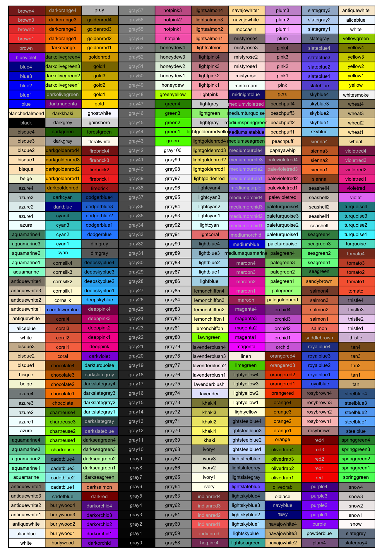
While the default colors may be fine for many applications, they are often not sufficient to highlight the relationships of interest or are not optimal for the intended audience/publication. For our boxplot, the default colors look great but still we may want some freedom with customization.
There are “cheatsheets” available for specifying the base R colors by name or hexadecimal code, and there are these websites here and here for picking colors or palettes of interest and returning the hexadecimal code(s).
To apply any of these colors to our plot, we can individually specify
the colors by providing them within a scale_fill_manual
layer.
Select two colors that speak to you
Add these colors into the code using
scale_fill_manual.
example:
scale_colour_manual(values = c("red", "blue", "green"))
This line can be inserted before
facet_grid()
# plotting IL-6

IL6 <- plotCounts(dds,
                  gene="ENSMUSG00000025746.11",
                  intgroup = c("Treatment", "Genotype"),
                  returnData = TRUE) |>
  ggplot(aes(x = Treatment,
             y = count,
             fill = Treatment)) +
  geom_boxplot(outlier.shape = NA, color = "black") +
  geom_jitter(shape = 16, position = position_jitter(0.2)) +
  labs(title = "IL6 expression",
       y = "Normalized counts",
       x = "Treatment") +
  theme_grey() +
  theme(plot.title = element_text(hjust = 0.5),
        axis.text = element_text(size = 8),
        axis.title = element_text(size = 14)) +
  scale_fill_manual(values = c("#f1a340", "#998ec3")) +
  facet_grid(~Genotype)

IL6
Step5: Complete Themes
ggplot2 provides complete themes which control all
non-data display. We have been using theme() to tweak the
display of an existing theme theme_grey().
More themes can be found here: https://ggplot2.tidyverse.org/reference/ggtheme.html
# plotting IL-6

IL6 <- plotCounts(dds,
                  gene="ENSMUSG00000025746.11",
                  intgroup = c("Treatment", "Genotype"),
                  returnData = TRUE) |>
  ggplot(aes(x = Treatment,
             y = count,
             fill = Treatment)) +
  geom_boxplot(outlier.shape = NA, color = "black") +
  geom_jitter(shape = 16, position = position_jitter(0.2)) +
  labs(title = "IL6 expression",
       y = "Normalized counts",
       x = "Treatment") +
  theme_linedraw() +
  theme(plot.title = element_text(hjust = 0.5),
        axis.text = element_text(size = 8),
        axis.title = element_text(size = 10)) +
  scale_fill_manual(values = c("#f1a340", "#998ec3")) +
  facet_grid(~Genotype)

IL6
Scenario: Stacey, an undergraduate in the Kremenstov lab, knows that Nos2 — a gene that encodes inducible nitric oxide synthase (iNOS)— plays a role in regulating the survival and metabolism of BMDCs (bone marrow-derived dendritic cells). She hypothesizes that, like IL-6, Nos2 expression will be upregulated in LPS-stimulated BMDCs compared to untreated cells. However, she wonders whether this expression will be reduced in BMDCs taken from PWD mice. Help Stacey visualize Nos2 expression to test her hypothesis. Output the results as a PDF (height = 2.5, width = 6).
# plotting Nos2What is dev.off()?
In R, when you create a plot that goes to a file (like a PDF, PNG, or SVG), you first open a graphics device (e.g., pdf(“plot.pdf”)). This tells R to start sending any plotting commands to that file.
dev.off() closes the graphics device, which:
- Finalizes and saves the file.
- Releases the connection to that device.
- Returns plotting back to your RStudio plotting window (or wherever it was before).
The pdf() function must come before the plotting
function (ex.plot() or plotCounts()). R by
default will send the plot to the file being created with
pdf(). You will get a blank PDF if the file was opened by
R, after the plot was created as the file never received any
information.
Session info
sessionInfo()## R version 4.5.3 (2026-03-11)
## Platform: x86_64-apple-darwin20
## Running under: macOS Tahoe 26.3.1
##
## Matrix products: default
## BLAS: /Library/Frameworks/R.framework/Versions/4.5-x86_64/Resources/lib/libRblas.0.dylib
## LAPACK: /Library/Frameworks/R.framework/Versions/4.5-x86_64/Resources/lib/libRlapack.dylib; LAPACK version 3.12.1
##
## locale:
## [1] en_US.UTF-8/en_US.UTF-8/en_US.UTF-8/C/en_US.UTF-8/en_US.UTF-8
##
## time zone: America/New_York
## tzcode source: internal
##
## attached base packages:
## [1] stats4 stats graphics grDevices utils datasets methods
## [8] base
##
## other attached packages:
## [1] fstcore_0.10.0 ggplotify_0.1.3
## [3] patchwork_1.3.2 pathview_1.50.0
## [5] msigdbr_25.1.1 cowplot_1.2.0
## [7] knitr_1.51 enrichplot_1.30.4
## [9] ggnewscale_0.5.2 DOSE_4.4.0
## [11] clusterProfiler_4.18.4 EnhancedVolcano_1.28.2
## [13] ggrepel_0.9.6 RColorBrewer_1.1-3
## [15] pheatmap_1.0.13 genekitr_1.2.8
## [17] ggplot2_4.0.1 tidyr_1.3.2
## [19] dplyr_1.1.4 DESeq2_1.50.2
## [21] SummarizedExperiment_1.40.0 Biobase_2.70.0
## [23] MatrixGenerics_1.22.0 matrixStats_1.5.0
## [25] GenomicRanges_1.62.1 Seqinfo_1.0.0
## [27] IRanges_2.44.0 S4Vectors_0.48.0
## [29] BiocGenerics_0.56.0 generics_0.1.4
##
## loaded via a namespace (and not attached):
## [1] splines_4.5.3 bitops_1.0-9 urltools_1.7.3.1
## [4] tibble_3.3.1 R.oo_1.27.1 triebeard_0.4.1
## [7] polyclip_1.10-7 graph_1.88.1 XML_3.99-0.20
## [10] lifecycle_1.0.5 mixsqp_0.3-54 lattice_0.22-9
## [13] MASS_7.3-65 magrittr_2.0.4 openxlsx_4.2.8.1
## [16] sass_0.4.10 rmarkdown_2.30 jquerylib_0.1.4
## [19] yaml_2.3.12 remotes_2.5.0 otel_0.2.0
## [22] ggtangle_0.1.1 zip_2.3.3 sessioninfo_1.2.3
## [25] pkgbuild_1.4.8 ggvenn_0.1.19 DBI_1.2.3
## [28] abind_1.4-8 pkgload_1.4.1 purrr_1.2.1
## [31] R.utils_2.13.0 RCurl_1.98-1.17 ggraph_2.2.2
## [34] yulab.utils_0.2.3 tweenr_2.0.3 rappdirs_0.3.4
## [37] gdtools_0.4.4 irlba_2.3.5.1 tidytree_0.4.7
## [40] codetools_0.2-20 DelayedArray_0.36.0 xml2_1.5.2
## [43] ggforce_0.5.0 tidyselect_1.2.1 aplot_0.2.9
## [46] farver_2.1.2 viridis_0.6.5 jsonlite_2.0.0
## [49] fst_0.9.8 ellipsis_0.3.2 tidygraph_1.3.1
## [52] systemfonts_1.3.1 tools_4.5.3 progress_1.2.3
## [55] treeio_1.34.0 Rcpp_1.1.1 glue_1.8.0
## [58] gridExtra_2.3 SparseArray_1.10.8 xfun_0.56
## [61] qvalue_2.42.0 usethis_3.2.1 withr_3.0.2
## [64] fastmap_1.2.0 truncnorm_1.0-9 digest_0.6.39
## [67] R6_2.6.1 gridGraphics_0.5-1 GO.db_3.22.0
## [70] RSQLite_2.4.5 R.methodsS3_1.8.2 fontLiberation_0.1.0
## [73] data.table_1.18.0 prettyunits_1.2.0 graphlayouts_1.2.2
## [76] httr_1.4.7 htmlwidgets_1.6.4 S4Arrays_1.10.1
## [79] scatterpie_0.2.6 pkgconfig_2.0.3 gtable_0.3.6
## [82] blob_1.3.0 S7_0.2.1 XVector_0.50.0
## [85] htmltools_0.5.9 fontBitstreamVera_0.1.1 geneset_0.2.7
## [88] fgsea_1.36.2 scales_1.4.0 png_0.1-8
## [91] ashr_2.2-63 ggfun_0.2.0 rstudioapi_0.18.0
## [94] reshape2_1.4.5 nlme_3.1-168 curl_7.0.0
## [97] org.Hs.eg.db_3.22.0 cachem_1.1.0 stringr_1.6.0
## [100] parallel_4.5.3 AnnotationDbi_1.72.0 pillar_1.11.1
## [103] grid_4.5.3 vctrs_0.7.0 tidydr_0.0.6
## [106] cluster_2.1.8.2 Rgraphviz_2.54.0 KEGGgraph_1.70.0
## [109] evaluate_1.0.5 invgamma_1.2 cli_3.6.5
## [112] locfit_1.5-9.12 compiler_4.5.3 rlang_1.1.7
## [115] crayon_1.5.3 SQUAREM_2021.1 labeling_0.4.3
## [118] plyr_1.8.9 fs_1.6.6 ggiraph_0.9.3
## [121] stringi_1.8.7 viridisLite_0.4.2 BiocParallel_1.44.0
## [124] assertthat_0.2.1 babelgene_22.9 Biostrings_2.78.0
## [127] lazyeval_0.2.2 devtools_2.4.6 pacman_0.5.1
## [130] GOSemSim_2.36.0 fontquiver_0.2.1 Matrix_1.7-4
## [133] europepmc_0.4.3 hms_1.1.4 bit64_4.6.0-1
## [136] KEGGREST_1.50.0 igraph_2.2.1 memoise_2.0.1
## [139] bslib_0.9.0 ggtree_4.0.4 fastmatch_1.1-8
## [142] bit_4.6.0 ape_5.8-1 gson_0.1.0Citation
title: “Analyzing RNA-Seq with DESeq2” author: “Michael I. Love, Simon Anders, and Wolfgang Huber”
Note: if you use DESeq2 in published research, please cite:
Love, M.I., Huber, W., Anders, S. (2014) Moderated estimation of fold change and dispersion for RNA-seq data with DESeq2. Genome Biology, 15:550. 10.1186/s13059-014-0550-8
Sabikunnahar, B., Snyder, J. P., Rodriguez, P. D., Sessions, K. J., Amiel, E., Frietze, S. E., & Krementsov, D. N. (2025). Natural genetic variation in wild-derived mice controls host survival and transcriptional responses during endotoxic shock. ImmunoHorizons, 9(5), vlaf007. https://doi.org/10.1093/immhor/vlaf007