Analyzing RNA-Seq Part III

Getting Started

Code chunk options

Install the required R libraries

# Install CRAN packages
#install.packages(c("knitr", "RColorBrewer", "pheatmap"))
#BiocManager::install("apeglm") # Update all/some/none? [a/s/n] - type n 
#install.packages("pacman")

Libraries loaded

# loading required packages 
pacman::p_load(DESeq2, dplyr, tidyr, ggplot2, genekitr, pheatmap, 
               RColorBrewer, EnhancedVolcano, clusterProfiler, DOSE, 
               ggnewscale, enrichplot, knitr, cowplot, msigdbr, pathview, 
               patchwork, ggplotify)

About the Data

For today’s lesson we will be working with RNA-seq data from another recent publication in ImmunoHorizons by Sabikunnahar et al. (2025).

Summary: Innate immune cells rapidly respond to microbial threats, but if unchecked, these responses can harm the host, as seen in septic shock. To explore how genetic variation influences these responses, researchers compared standard lab mice (C57BL/6) with genetically diverse wild-derived mice (PWD).

Experimental Design: The authors isolated bone marrow derived dendritic cells from B6, c11.2, and PWD mice and then either left them unstimulated or stimulated with LPS.

This experiment has:

Two treatments: untreated, LPS
Three genotypes: B6, c11.2, and PWD

The goal:

To test how LPS stimulation affects each genotype
Whether the response to LPS differs between genotype

`ENSM_partIII` folder contents

Contents of the ENSM_counts folder:

The normalized counts matrix called PWD-LPSvsB6-LPS_normalized_matrix.csv
Filtered table of DE Genes called PWD-LPSvsB6-LPS_DEG_list.csv
PWD_annotation.csv file we will use later for the heatmap section
dds.RDS file that contains the results of the DESeq2 analysis performed on Monday.

Load Data

Please load the normalized counts matrix and save in an object called LPSvsB6_full.

LPSvsB6_full <- read.csv("PWD-LPSvsB6-LPS_normalized_matrix.csv",
                         header = T)


#head(LPSvsB6_full)

RDS object

An .RDS file is a file format in R used to save a single R object—like a dataframe, a list, a model, a matrix, etc.—in a compact, portable way. It lets you save your progress at any point in an analysis, so you don’t have to rerun everything

Saving RDS object

#saveRDS(object, file = "")

You can also share the object with others!

Loading RDS object

#object_name <- readRDS(object_name_of_RDS)

Below, load the dds.RDS object.

dds <- readRDS("dds.RDS")

Using `plotCounts()` to generate boxplots

Figure 3 of the paper shows an increase in pro-inflammatory cytokine production in response to LPS, with a reduced release in PWD mice compared to B6 mice. To recreate this finding, we’ll use the plotCounts() function along with ggplot2.

Step1: Find the Ensembl ID for IL-6. We’re interested in visualizing IL-6 expression. However, the dds object stores genes using Ensembl IDs with version numbers (e.g., “ENSMUSG00000054221.11”).

To find the correct ID for IL-6:

Search the result_LPS_compare data frame for the Ensembl ID (with version) that corresponds to IL-6.
Write the full Ensembl ID (including version) below:

# Type the ENSMUSG ID (with version) for IL-6 here:

Step2: Use the plotCounts() function to generate a plot of normalized counts for the IL-6 gene. Check the help page (?plotCounts) to understand the function and its arguments.

Set the grouping variable with: intgroup = c("Treatment", "Genotype"). This will allow you to see how IL-6 expression varies across treatment conditions and genotypes.
Set returnData = TRUE

?plotCounts

plot_IL6 <- plotCounts(dds, 
                       gene="ENSMUSG00000025746.11", 
                       intgroup = c("Treatment", "Genotype"),
                       returnData = TRUE)

Step3: Now we are ready to output the results to ggplot() to add custom aesthetics.

# plotting IL-6

IL6 <- plotCounts(dds, 
                  gene="ENSMUSG00000025746.11", 
                  intgroup = c("Treatment", "Genotype"),  
                  returnData = TRUE) |> 
  ggplot(aes(x = Treatment, 
             y = count, 
             fill = Treatment)) + 
  geom_boxplot(outlier.shape = NA, color = "black") + 
  geom_jitter(shape = 16, position = position_jitter(0.2)) +
  labs(title = "IL6 expression", 
       y = "Normalized counts", 
       x = "Treatment") + 
  theme_grey() + 
  theme(plot.title = element_text(hjust = 0.5),
        axis.text = element_text(size = 8),
        axis.title = element_text(size = 14)) +
  facet_grid(~Genotype)

IL6

Step4: Color scales

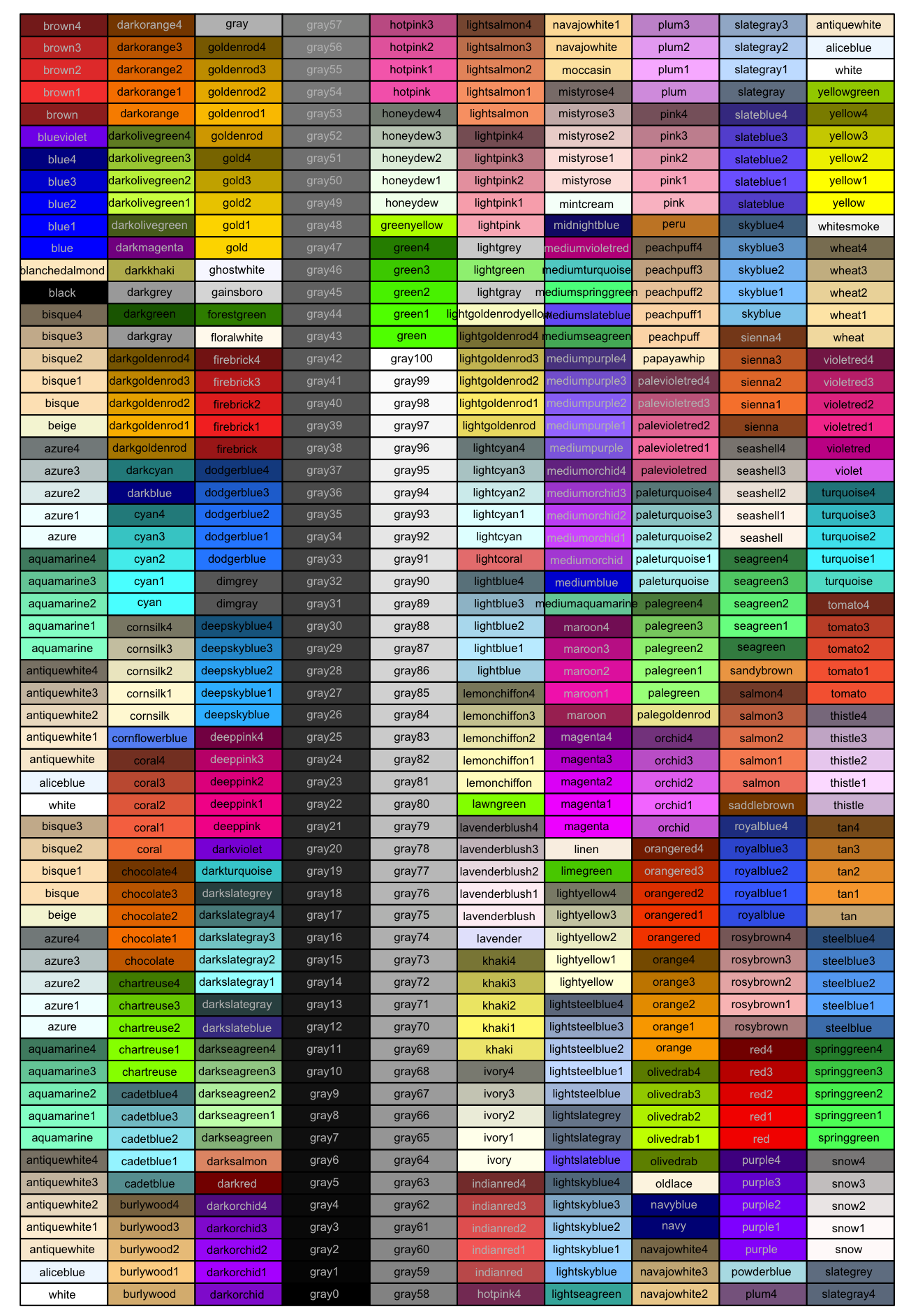
While the default colors may be fine for many applications, they are often not sufficient to highlight the relationships of interest or are not optimal for the intended audience/publication. For our boxplot, the default colors look great but still we may want some freedom with customization.

There are “cheatsheets” available for specifying the base R colors by name or hexadecimal code, and there are these websites here and here for picking colors or palettes of interest and returning the hexadecimal code(s).

To apply any of these colors to our plot, we can individually specify the colors by providing them within a scale_fill_manual layer.

Select two colors that speak to you
Add these colors into the code using scale_fill_manual.

example: scale_colour_manual(values = c("red", "blue", "green"))

This line can be inserted before facet_grid()

# plotting IL-6

IL6 <- plotCounts(dds, 
                  gene="ENSMUSG00000025746.11", 
                  intgroup = c("Treatment", "Genotype"),  
                  returnData = TRUE) |> 
  ggplot(aes(x = Treatment, 
             y = count, 
             fill = Treatment)) + 
  geom_boxplot(outlier.shape = NA, color = "black") + 
  geom_jitter(shape = 16, position = position_jitter(0.2)) +
  labs(title = "IL6 expression", 
       y = "Normalized counts", 
       x = "Treatment") + 
  theme_grey() + 
  theme(plot.title = element_text(hjust = 0.5),
        axis.text = element_text(size = 8),
        axis.title = element_text(size = 14)) +
  scale_fill_manual(values = c("#f1a340", "#998ec3")) +
  facet_grid(~Genotype)

IL6

Step5: Complete Themes

ggplot2 provides complete themes which control all non-data display. We have been using theme() to tweak the display of an existing theme theme_grey().

More themes can be found here: https://ggplot2.tidyverse.org/reference/ggtheme.html

# plotting IL-6

IL6 <- plotCounts(dds, 
                  gene="ENSMUSG00000025746.11", 
                  intgroup = c("Treatment", "Genotype"),  
                  returnData = TRUE) |> 
  ggplot(aes(x = Treatment, 
             y = count, 
             fill = Treatment)) + 
  geom_boxplot(outlier.shape = NA, color = "black") + 
  geom_jitter(shape = 16, position = position_jitter(0.2)) +
  labs(title = "IL6 expression", 
       y = "Normalized counts", 
       x = "Treatment") + 
  theme_linedraw() + 
  theme(plot.title = element_text(hjust = 0.5),
        axis.text = element_text(size = 8),
        axis.title = element_text(size = 10)) +
  scale_fill_manual(values = c("#f1a340", "#998ec3")) +
  facet_grid(~Genotype)

IL6

Scenario: Stacey, an undergraduate in the Kremenstov lab, knows that Nos2 — a gene that encodes inducible nitric oxide synthase (iNOS)— plays a role in regulating the survival and metabolism of BMDCs (bone marrow-derived dendritic cells). She hypothesizes that, like Il6, Nos2 expression will be upregulated in LPS-stimulated BMDCs compared to untreated cells. However, she wonders whether this expression will be reduced in BMDCs taken from PWD mice. Help Stacey visualize Nos2 expression to test her hypothesis. Output the results as a PDF (height = 2.5, width = 6).

#pdf(file = "Nos2_boxplot.pdf", height = 2.5, width = 6)

# plotting Nos2

Nos2 <- plotCounts(dds, 
               gene="ENSMUSG00000020826.9", 
               intgroup = c("Treatment", "Genotype"),  
               returnData = TRUE) |> 
  ggplot(aes(x = Treatment, y = count, fill = Treatment)) + 
  geom_boxplot(outlier.shape = NA, color = "black") + 
  geom_jitter(shape = 16, position = position_jitter(0.2)) +
  labs(title = "Nos2 expression", 
       y = "Normalized counts", 
       x = "Treatment") + 
  theme_linedraw() + 
  theme(plot.title = element_text(hjust = 0.5),
        axis.text = element_text(size = 8),
        axis.title = element_text(size = 10)) +
  scale_fill_manual(values = c("black", "red")) + 
  facet_grid(~Genotype)

Nos2

#dev.off()

What is `dev.off()`?

In R, when you create a plot that goes to a file (like a PDF, PNG, or SVG), you first open a graphics device (e.g., pdf(“plot.pdf”)). This tells R to start sending any plotting commands to that file.

dev.off() closes the graphics device, which:

Finalizes and saves the file.
Releases the connection to that device.
Returns plotting back to your RStudio plotting window (or wherever it was before).

The pdf() function must come before the plotting function (ex.plot() or plotCounts()). R by default will send the plot to the file being created with pdf(). You will get a blank PDF if the file was opened by R, after the plot was created as the file never received any information.

Introduction to Heatmaps

We have discovered that ggplot2 has incredible functionality and versatility; however, it is not always the best choice for all graphics. There are a plethora of different packages that specialize in particular types of figures. Today we will concentrate on creating hierarchical heatmaps using one of these packages called pheatmap.

pheatmap is a package used for drawing pretty heatmaps in R. This function has several advantages including the ability to control heatmap dimensions and appearance.

#install.packages(pheatmap) #install pheatmap 
library(pheatmap)

Applying `dplyr` to heatmap generation

`dplyr` basics

The first argument is always a data frame.
The subsequent arguments typically describe which columns/rows to operate on, using the variable name.
The output is always a new data frame.

Common verbs from `dpylr`

filter() allows you to keep rows based on the values of the columns.
summarise() reduces multiple values down to a single summary.
arrange() changes the ordering of the rows.
slice_head() and slice_tail() select the first or last rows.
mutate() adds new variables that are functions of existing variables
select() picks variables based on their names.

Step 1 Load the DE matrix. containing list of DEGs into an object called deg_matrix. After loading, make sure that deg_matrix is being read as data frame.

deg_matrix <- read.csv("PWD-LPSvsB6-LPS_DEG_list.csv", header = T)
deg_matrix <- data.frame(deg_matrix)

Step 2 Selecting columns of interest.

heatmap_matrix <- select(deg_matrix, 
                         symbol, 
                         Unstim_B6_Rep1:LPS_PWD_Rep4)

heatmap_matrix <- data.frame(heatmap_matrix, row.names = 1)

Step 3 Read in annotation file called PWD_annotation.csv.

heatmap_anno <- read.csv("PWD_annotation.csv", header = T)
heatmap_anno

##            sample_id genotype    treatment
## 1     Unstim_B6_Rep1       B6 Unstimulated
## 2     Unstim_B6_Rep2       B6 Unstimulated
## 3     Unstim_B6_Rep3       B6 Unstimulated
## 4     Unstim_B6_Rep4       B6 Unstimulated
## 5  Unstim_c11.2_rep1    c11.2 Unstimulated
## 6  Unstim_c11.2_rep2    c11.2 Unstimulated
## 7  Unstim_c11.2_rep3    c11.2 Unstimulated
## 8  Unstim_c11.2_rep4    c11.2 Unstimulated
## 9    Unstim_PWD_rep1      PWD Unstimulated
## 10   Unstim_PWD_rep2      PWD Unstimulated
## 11   Unstim_PWD_rep3      PWD Unstimulated
## 12   Unstim_PWD_rep4      PWD Unstimulated
## 13       LPS_B6_rep1       B6          LPS
## 14       LPS_B6_rep2       B6          LPS
## 15       LPS_B6_rep3       B6          LPS
## 16       LPS_B6_rep4       B6          LPS
## 17    LPS_c11.2_Rep1    c11.2          LPS
## 18    LPS_c11.2_Rep2    c11.2          LPS
## 19    LPS_c11.2_Rep3    c11.2          LPS
## 20    LPS_c11.2_Rep4    c11.2          LPS
## 21      LPS_PWD_Rep1      PWD          LPS
## 22      LPS_PWD_Rep2      PWD          LPS
## 23      LPS_PWD_Rep3      PWD          LPS
## 24      LPS_PWD_Rep4      PWD          LPS

Step 4 Assign the sample names to be the row names.

The row names in the annotation file need to be read as sample names and also match the column names of our counts data. Then we will “select” the genotype and treatment column.

# Assign the sample names to be the row names
rownames(heatmap_anno) <- heatmap_anno$sample_id

heatmap_anno <- select(heatmap_anno, genotype, treatment)

The object heatmap_anno will be the data frame for the column annotations.
If you wanted to add more column annotations, this is the point during the workflow that you would do it.

Step 5 Assign factor levels

Factor levels will determine the color automatically assigned to the group. We can manually specify the levels using the factor() function.

# Re-level factors
heatmap_anno$genotype <- factor(heatmap_anno$genotype, 
                                levels = c("B6", "c11.2", "PWD"))

heatmap_anno$treatment <- factor(heatmap_anno$treatment, 
                                levels = c("Unstimulated", "LPS"))

Step 5 Provide customized colors

You can define customized colors to display the heatmap using the brewer.pal() function from the RColorBrewer package. For example:

# Colors for heatmap
heatmap_colors <- rev(brewer.pal(10, "RdBu"))

This creates a red-to-blue color gradient with 10 shades, and rev() reverses the order so that red represents higher values and blue represents lower values (or vice versa, depending on your data).

You can also specify custom colors for the annotations (e.g., for sample groups or conditions). These colors need to be provided as a named list, where each element matches the annotation values.

# Colors for denoting annotations
ann_colors <- list(genotype = c(B6 = "#7fc97f", 
                                c11.2 = "#beaed4", 
                                PWD = "#fdc086" ),
                   treatment = c(Unstimulated = "#a6cee3",
                                 LPS = "#1f78b4"))

# Based on the colorbrewer2 
# https://colorbrewer2.org/#type=qualitative&scheme=Paired&n=3

Plotting with `pheatmap`

Below, are the major arguments required to plot with pheatmap.

# BASIC USAGE 
## DO NOT RUN 
#pheatmap(numeric_matrix, 
         #color = ,
         #annotation_col = , 
         #annotation_colors = ,
         #show_colnames = , 
         #show_rownames = )

?pheatmap() #if you have questions 
# We would like to remove column names and row names 
# color = A custom color palette to represent heatmap values 
# annotation_col = Adds metadata about the columns (samples), such as treatment group, time point, etc.
# annotation_color = Tells pheatmap how to color those annotations (e.g., red for "treated", blue for "control").
#show_colnames = shows/hides column names.
#show_rownames = shows/hides column names.

Using the information outlined above and in your global environment, fill in the (6) arguments required.

pheatmap(heatmap_matrix, 
         color = heatmap_colors,
         annotation_col = heatmap_anno,
         annotation_colors = ann_colors,
         show_colnames = F, 
         show_rownames = F)

Transforming the Data: Z-score

When you add scale = "row" in pheatmap(), the heatmap displays Z-scores instead of the original normalized count values.

Z-scores are calculated gene by gene by subtracting the mean and dividing by the standard deviation for each row.

This transformation is applied after clustering, so it doesn’t affect how rows or columns are grouped. Instead, it improves the visual contrast by standardizing each gene’s range of expression.

This is especially helpful when you want to highlight relative differences within each gene across samples, rather than comparing absolute expression values between genes.

pheatmap(heatmap_matrix, 
         color = heatmap_colors,
         annotation_col = heatmap_anno,
         annotation_colors = ann_colors,
         show_colnames = F, 
         show_rownames = F,
         scale = "row")

Major Take-away Some genes or features have naturally higher values than others—but that doesn’t mean they’re more important!

If you don’t scale, the clustering might group samples based on just the genes with the biggest raw numbers, rather than patterns of change.

Let’s add a few more arguments:

pheatmap(heatmap_matrix, 
         color = heatmap_colors,
         annotation_col = heatmap_anno,
         annotation_colors = ann_colors,
         show_colnames = F, 
         show_rownames = F,
         scale = "row",
         annotation_names_col = F,
         clustering_distance_cols = "euclidean", 
         clustering_method = "complete")

#cutree_rows = 4

What is Hierarchical Clustering?

Hierarchical clustering is a method for grouping similar “things” together based on how close they are to each other.

clustering_distance_cols = "euclidean"

This sets the distance metric for clustering the columns. It is asking, “How similar are these samples based on their overall expression patterns?”
Good default; works well with scaled data.

clustering_method = "complete"

This defines the method used to link clusters together in hierarchical clustering.
Tends to produce compact, tight clusters; default and reliable choice.

Output heatmap as PDF

Next, we will convert this plot into a ggplot object and save it into heatmap_final.

Go ahead and save heatmap_final as a PDF, width = 5, height =6.

#pdf(heatmap_final, file = "heatmap_PWD-LPSvsB6-LPS.pdf", width = 5, height = 6)

heatmap_final <- as.ggplot(pheatmap(heatmap_matrix, 
                              color = heatmap_colors,
                              annotation_col = heatmap_anno,
                              annotation_colors = ann_colors,
                              show_colnames = F, 
                              show_rownames = F,
                              scale = "row",
                              annotation_names_col = F,
                              clustering_distance_cols = "euclidean",
                              clustering_method = "complete",
                              cutree_rows = 4))

#dev.off()

Last “Black Trail” Exercise

Scenario: Sam, another undergraduate in the Kremenstov lab, wants to visualize only the top 20 differentially expressed (DE) genes. Right now, the heatmap includes all 5,112 genes, which makes it hard to focus on specific genes of interest. Sam is especially interested in seeing whether Apobec3 is among the top 20.

Sam’s hypothesis: Apobec3 expression and function in dendritic cells differ between PWD and B6 mice, contributing to the differential immune responses observed in these strains.

Help Sam create a new heatmap that only displays the top 20 DE genes.

Hint: To create the heatmap for the top 20 genes, first, you need to arrange the rows by the adjusted p-value (padj). Then, select the top 20 rows of interest before creating the new top20_heatmap_matrix.

Session info

sessionInfo()

## R version 4.4.3 (2025-02-28)
## Platform: x86_64-apple-darwin20
## Running under: macOS Sequoia 15.3
## 
## Matrix products: default
## BLAS:   /Library/Frameworks/R.framework/Versions/4.4-x86_64/Resources/lib/libRblas.0.dylib 
## LAPACK: /Library/Frameworks/R.framework/Versions/4.4-x86_64/Resources/lib/libRlapack.dylib;  LAPACK version 3.12.0
## 
## locale:
## [1] en_US.UTF-8/en_US.UTF-8/en_US.UTF-8/C/en_US.UTF-8/en_US.UTF-8
## 
## time zone: America/New_York
## tzcode source: internal
## 
## attached base packages:
## [1] stats4    stats     graphics  grDevices utils     datasets  methods  
## [8] base     
## 
## other attached packages:
##  [1] ggplotify_0.1.2             patchwork_1.3.0            
##  [3] pathview_1.46.0             msigdbr_10.0.1             
##  [5] cowplot_1.1.3               knitr_1.50                 
##  [7] enrichplot_1.26.6           ggnewscale_0.5.1           
##  [9] DOSE_4.0.1                  clusterProfiler_4.14.6     
## [11] EnhancedVolcano_1.24.0      ggrepel_0.9.6              
## [13] RColorBrewer_1.1-3          pheatmap_1.0.12            
## [15] genekitr_1.2.8              ggplot2_3.5.1              
## [17] tidyr_1.3.1                 dplyr_1.1.4                
## [19] DESeq2_1.46.0               SummarizedExperiment_1.36.0
## [21] Biobase_2.66.0              MatrixGenerics_1.18.1      
## [23] matrixStats_1.5.0           GenomicRanges_1.58.0       
## [25] GenomeInfoDb_1.42.3         IRanges_2.40.1             
## [27] S4Vectors_0.44.0            BiocGenerics_0.52.0        
## 
## loaded via a namespace (and not attached):
##   [1] splines_4.4.3           later_1.4.1             bitops_1.0-9           
##   [4] urltools_1.7.3          tibble_3.2.1            R.oo_1.27.0            
##   [7] triebeard_0.4.1         polyclip_1.10-7         graph_1.84.1           
##  [10] XML_3.99-0.18           lifecycle_1.0.4         lattice_0.22-6         
##  [13] MASS_7.3-65             magrittr_2.0.3          openxlsx_4.2.8         
##  [16] sass_0.4.9              rmarkdown_2.29          jquerylib_0.1.4        
##  [19] yaml_2.3.10             remotes_2.5.0           httpuv_1.6.15          
##  [22] ggtangle_0.0.6          zip_2.3.2               sessioninfo_1.2.3      
##  [25] pkgbuild_1.4.7          ggvenn_0.1.10           DBI_1.2.3              
##  [28] abind_1.4-8             pkgload_1.4.0           zlibbioc_1.52.0        
##  [31] purrr_1.0.4             R.utils_2.13.0          RCurl_1.98-1.17        
##  [34] ggraph_2.2.1            yulab.utils_0.2.0       tweenr_2.0.3           
##  [37] GenomeInfoDbData_1.2.13 tidytree_0.4.6          codetools_0.2-20       
##  [40] DelayedArray_0.32.0     xml2_1.3.8              ggforce_0.4.2          
##  [43] tidyselect_1.2.1        aplot_0.2.5             UCSC.utils_1.2.0       
##  [46] farver_2.1.2            viridis_0.6.5           rmdformats_1.0.4       
##  [49] jsonlite_2.0.0          ellipsis_0.3.2          tidygraph_1.3.1        
##  [52] tools_4.4.3             progress_1.2.3          treeio_1.30.0          
##  [55] Rcpp_1.0.14             glue_1.8.0              gridExtra_2.3          
##  [58] SparseArray_1.6.2       xfun_0.51               qvalue_2.38.0          
##  [61] usethis_3.1.0           withr_3.0.2             fastmap_1.2.0          
##  [64] digest_0.6.37           R6_2.6.1                mime_0.13              
##  [67] gridGraphics_0.5-1      colorspace_2.1-1        GO.db_3.20.0           
##  [70] RSQLite_2.3.9           R.methodsS3_1.8.2       generics_0.1.3         
##  [73] data.table_1.17.0       prettyunits_1.2.0       graphlayouts_1.2.2     
##  [76] httr_1.4.7              htmlwidgets_1.6.4       S4Arrays_1.6.0         
##  [79] pkgconfig_2.0.3         gtable_0.3.6            blob_1.2.4             
##  [82] XVector_0.46.0          htmltools_0.5.8.1       geneset_0.2.7          
##  [85] profvis_0.4.0           bookdown_0.42           fgsea_1.32.0           
##  [88] scales_1.3.0            png_0.1-8               ggfun_0.1.8            
##  [91] rstudioapi_0.17.1       reshape2_1.4.4          nlme_3.1-168           
##  [94] org.Hs.eg.db_3.20.0     cachem_1.1.0            stringr_1.5.1          
##  [97] parallel_4.4.3          miniUI_0.1.1.1          AnnotationDbi_1.68.0   
## [100] pillar_1.10.1           grid_4.4.3              vctrs_0.6.5            
## [103] urlchecker_1.0.1        promises_1.3.2          xtable_1.8-4           
## [106] Rgraphviz_2.50.0        evaluate_1.0.3          KEGGgraph_1.66.0       
## [109] cli_3.6.4               locfit_1.5-9.12         compiler_4.4.3         
## [112] rlang_1.1.5             crayon_1.5.3            labeling_0.4.3         
## [115] plyr_1.8.9              fs_1.6.5                stringi_1.8.7          
## [118] viridisLite_0.4.2       BiocParallel_1.40.0     assertthat_0.2.1       
## [121] babelgene_22.9          munsell_0.5.1           Biostrings_2.74.1      
## [124] lazyeval_0.2.2          devtools_2.4.5          pacman_0.5.1           
## [127] GOSemSim_2.32.0         Matrix_1.7-3            europepmc_0.4.3        
## [130] hms_1.1.3               bit64_4.6.0-1           KEGGREST_1.46.0        
## [133] shiny_1.10.0            igraph_2.1.4            memoise_2.0.1          
## [136] bslib_0.9.0             ggtree_3.14.0           fastmatch_1.1-6        
## [139] bit_4.6.0               ape_5.8-1               gson_0.1.0

Citation

title: “Analyzing RNA-Seq with DESeq2” author: “Michael I. Love, Simon Anders, and Wolfgang Huber”

Note: if you use DESeq2 in published research, please cite:

Love, M.I., Huber, W., Anders, S. (2014) Moderated estimation of fold change and dispersion for RNA-seq data with DESeq2. Genome Biology, 15:550. 10.1186/s13059-014-0550-8

Sabikunnahar, B., Snyder, J. P., Rodriguez, P. D., Sessions, K. J., Amiel, E., Frietze, S. E., & Krementsov, D. N. (2025). Natural genetic variation in wild-derived mice controls host survival and transcriptional responses during endotoxic shock. ImmunoHorizons, 9(5), vlaf007. https://doi.org/10.1093/immhor/vlaf007

Analyzing RNA-Seq Part III